State Space Modeling for Estimating Team Strength and Home Advantage
We are interested in modeling team strength over the length of a season. The strength metric will not be static as it evolves over the course of the season due to factors such as injuries, confidence and the ability of opposition teams to figure out how to play against a team. Therefore we are interested in modeling team strength as a time series.
The data used in order to model team strength is betting data from the website https://www.bet365.com/en/
Game by game odds for all the leagues used to demonstrate the model were obtained from http://www.football-data.co.uk/
The model is an implementation of the paper presented here https://arxiv.org/pdf/1701.05976.pdf
From the accompanying blog post:
“Moreso than wins and losses or point differential, perhaps the best game-level metric of team strength comes not in what happens during the game, but what’s known before the game begins. Indeed, it’s been shown time and again that there’s no better way to judge models in sports than to compare to betting market data. Prior to each contest, betting markets put out probabilities associated with each team winning. The reason this data is so accurate is that it takes into account all of the factors above – injuries, opponent strength, line-ups, tanking, etc.”
Model
Betting data comes in the form of weekly odds of a home win, draw or loss.
Let $y_{i,j,w} = logit ( p_{i,j,w} ) $ be the log odds of observed probability of a home win for team i against team j in week w.
We can model $ E [ logit (p_{i,j,w} ] = \theta_{i,w} - \theta_{j,w} + \alpha + \alpha_{Ti} $
where: $
\begin{align}
\theta_{i,w} &: \text{team strength rating of team i in week w}
\theta_{j,w} &: \text{team strength rating of team j in week w}
\alpha &: \text{baseline home advtange for all teams}
\alpha_{Ti} &: \text{home advantage of team i}
\text{For any team i we can assume that the team strength in week w is given as follows:}
\theta_{i,w} & \sim N(\gamma\theta_{i, w-1}, \tau_{w}^2)
\text{where: }
\theta_{i,w-1} &: \text{team strength for team i in week w-1}
\gamma &: \text{autocorrelation at order 1 for team strength in week w}
\tau_{w} &: \text{week-level uncertainity in the evolution of team strength} \
\end{align} $
Implementation in Stan
Some Helper Functions
import pystan
def logit(p):
    return np.log(p/(1-p))
def prepare_data(filename):

    df = pd.read_csv(filename, dayfirst = True)

    df = df[['Date', 'HomeTeam', 'AwayTeam', 'B365H', 'B365D', 'B365A']]

    df['p_home'] = (1/df['B365H'])

    df['Date'] = pd.to_datetime(df['Date'], dayfirst = True)

    df['week'] = (np.floor((df['Date'] - df['Date'][0])/np.timedelta64(1, 'W'))).astype('int') + 1

    return df
def prepare_model_data(df):
    '''
    returns a dictionary that will be passed to the stan model
    '''

    model_data = {}

    Teams =  sorted(list(df['HomeTeam'].unique()))

    model_data['nteams'] = len(Teams)

    model_data['nweeks'] = max(df['week']) + 1

    model_data['n'] = len(df)
    model_data['ht'] = []

    X = np.zeros((len(Teams), df.shape[0]))

    for i in range(0, df.shape[0]):
        X[Teams.index(df.loc[i, 'HomeTeam']), i ] = 1
        X[Teams.index(df.loc[i, 'AwayTeam']), i] = -1
        model_data['ht'].append(Teams.index(df.loc[i, 'HomeTeam']) + 1)

    model_data['X'] = X

    model_data['y'] = logit(df['p_home'])

    model_data['w'] = df['week']

    return model_data, Teams
def plot_params():
return fit.plot(pars = ['alpha', 'gammaWeek'])
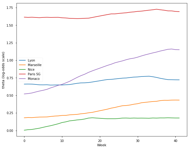
def plot_team_strengths(sample, l, Teams):
plt.figure(figsize = (10,8))
for i in l:
id = Teams.index(i)
plt.plot(sample['theta'][1000:, :, id].mean(axis = 0))
plt.xlabel('Week')
plt.ylabel('theta (log-odds scale)')
plt.legend(l)
def get_results(filename, l):

    df = prepare_data(filename)
    model_data, Teams = prepare_model_data(df)

    fit = pystan.stan(model_code=data + parameters + transformed_params + model, data=model_data, iter=3000, warmup = 1000, chains=2)

    sample= fit.extract(permuted = True)
    plot_team_strengths(sample, l, Teams)

    return sample, Teams
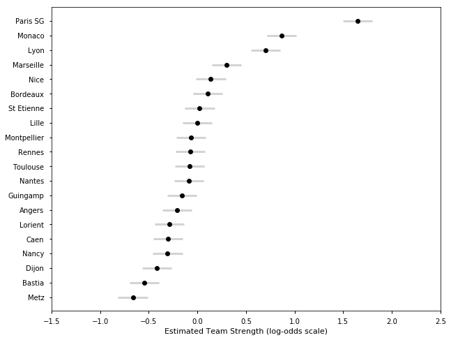
def plot_final_rating(samples, Teams):

    x = samples['theta'][1000:][35:][:].mean(axis = 0).mean(axis=0)
    e = samples['theta'][1000:][35:][:].std(axis = 0).mean(axis=0)

    data = sorted(list(zip(x, Teams, e)), key = lambda x: x[0])
    x_val = [x[0] for x in data]
    e_val = [x[2] for x in data]
    Teams = [x[1] for x in data]

    y = np.linspace(-2.0, 2.0, len(x_val))
    x = x_val
    my_yticks = Teams
    plt.figure(figsize = (10,8))
    plt.yticks(y, my_yticks)
    plt.errorbar(x, y, xerr = e_val, fmt='o', color='black',
             ecolor='lightgray', elinewidth=3, capsize=0)
    plt.xlabel('Estimated Team Strength (log-odds scale)')
    plt.xlim(-1.5,2.5)
    plt.show()
Stan Implementation
We need a matrix of dimensions W,N that contains the weekly strength rating for each team.
data = """
data {
    int<lower=0> n;      // total number of games
    int<lower=0> nweeks; // total number of weeks
    int<lower=0> nteams; // total number of teams
    int<lower=0> w[n];
    vector[n] y;
    int<lower=0> ht[n];
    matrix[nteams, n] X;
}
"""
parameters = """
parameters {
    real<lower = 0, upper=1> gammaWeek; // autoregressive coefficient
    real<lower = 0> tauSeason;  // uncertainty in team strength from season to season
    real<lower = 0> tauWeek; // uncertainty in team strength from week to week
    real<lower = 0> tauGame; // uncertainty in team strength from game to game
    real alpha; // baseline home strength
    vector[nteams] alphaTeam; // home strength for each team
    matrix[nweeks, nteams] theta;
}
"""
transformed_params = """
transformed parameters {
    vector[n] mu;
    for (i in 1:n) {
        mu[i] <- alpha + theta[w[i],:] * X[:,i] + alphaTeam[ht[i]];
    }
 }
"""
model = """
model {
    alpha ~ normal(0.01, 0.005);
    gammaWeek ~ normal(0.9, 0.05);
    tauSeason ~ student_t(20, 0, 1);
    tauWeek ~ student_t(5, 0, 1);
    tauGame ~ student_t(5, 0, 1);

    y ~ normal(mu, tauGame);

    for (j in 1: nteams){
        alphaTeam ~ normal(0.1, 0.1);
    }
    for (j in 1:nteams){
        theta[1,j] ~ normal(0, tauSeason);
    }

    for (www in 2:nweeks) {
        for (j in 1:nteams) {
            theta[www,j] ~ normal(gammaWeek*theta[www-1,j], tauWeek);
          }

     }
    }
"""
Barclays Premier League Season 2017-18
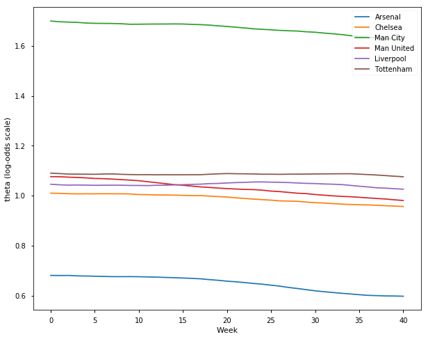
l = ['Arsenal', 'Chelsea', 'Man City', 'Man United', 'Liverpool', 'Tottenham']
## let's look at the weekly time series of team strengths for these six teams
samplesE1718, TeamsE1718 = get_results('E02017.csv', l)
INFO:pystan:COMPILING THE C++ CODE FOR MODEL anon_model_7eab52f40be587905f219e2d7f11fcab NOW.
WARNING:pystan:Rhat for parameter tauWeek is 1.642752747457723!
WARNING:pystan:Rhat for parameter lp__ is 1.6266023276293617!
WARNING:pystan:Rhat above 1.1 or below 0.9 indicates that the chains very likely have not mixed
WARNING:pystan:3145 of 4000 iterations saturated the maximum tree depth of 10 (78.625%)
WARNING:pystan:Run again with max_treedepth larger than 10 to avoid saturation
WARNING:pystan:Chain 1: E-BFMI = 0.005175413428662303
WARNING:pystan:Chain 2: E-BFMI = 0.004273288134546748
WARNING:pystan:E-BFMI below 0.2 indicates you may need to reparameterize your model
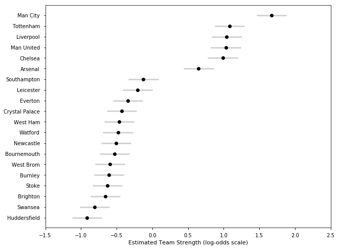
## Let's look at the estimated team strengths
plot_final_rating(samplesE1718, TeamsE1718)
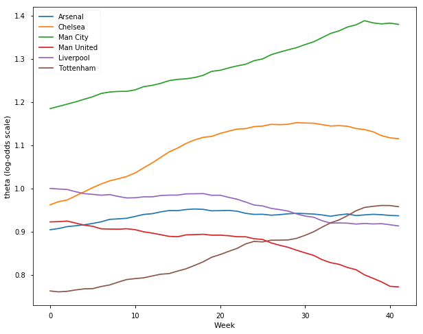
## Premier League Season 2016-17
samplesE1617, TeamsE1617 = get_results('E0201617.csv', l)
INFO:pystan:COMPILING THE C++ CODE FOR MODEL anon_model_7eab52f40be587905f219e2d7f11fcab NOW.
WARNING:pystan:Rhat for parameter tauWeek is 1.1024429662692437!
WARNING:pystan:Rhat for parameter lp__ is 1.1385914195098517!
WARNING:pystan:Rhat above 1.1 or below 0.9 indicates that the chains very likely have not mixed
WARNING:pystan:134 of 4000 iterations saturated the maximum tree depth of 10 (3.35%)
WARNING:pystan:Run again with max_treedepth larger than 10 to avoid saturation
WARNING:pystan:Chain 1: E-BFMI = 0.012187576962741213
WARNING:pystan:Chain 2: E-BFMI = 0.030105243877863928
WARNING:pystan:E-BFMI below 0.2 indicates you may need to reparameterize your model
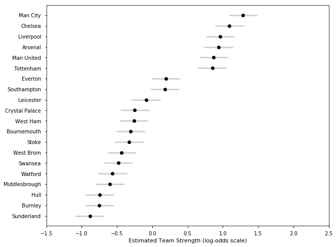
plot_final_rating(samplesE1617, TeamsE1617)
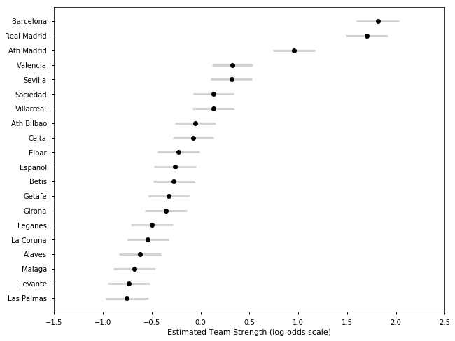
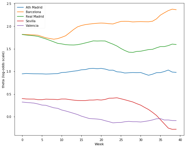
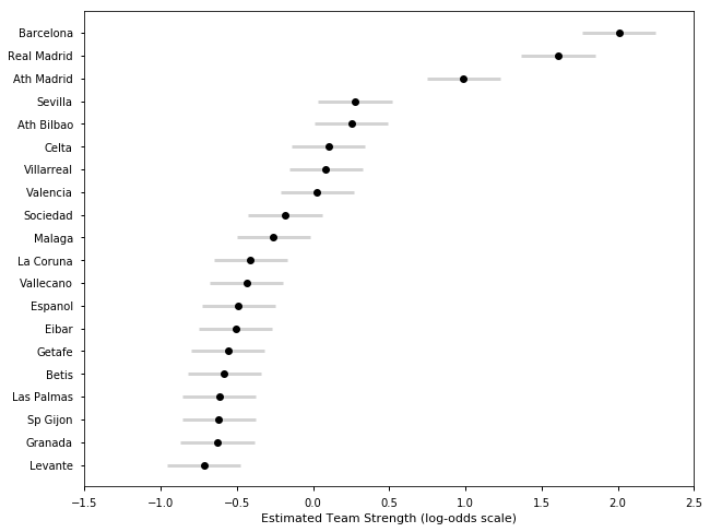
## Spanish La Liga Season 2017-18
l = ['Ath Madrid', 'Barcelona', 'Real Madrid', 'Sevilla', 'Valencia']
samplesS1718, TeamsS1718 = get_results('SP1718.csv', l)
INFO:pystan:COMPILING THE C++ CODE FOR MODEL anon_model_7eab52f40be587905f219e2d7f11fcab NOW.
WARNING:pystan:Rhat for parameter tauWeek is 1.512246483973463!
WARNING:pystan:Rhat for parameter lp__ is 1.5092250101486342!
WARNING:pystan:Rhat above 1.1 or below 0.9 indicates that the chains very likely have not mixed
WARNING:pystan:331 of 4000 iterations saturated the maximum tree depth of 10 (8.275%)
WARNING:pystan:Run again with max_treedepth larger than 10 to avoid saturation
WARNING:pystan:Chain 1: E-BFMI = 0.02979981850473017
WARNING:pystan:Chain 2: E-BFMI = 0.010154501598971476
WARNING:pystan:E-BFMI below 0.2 indicates you may need to reparameterize your model
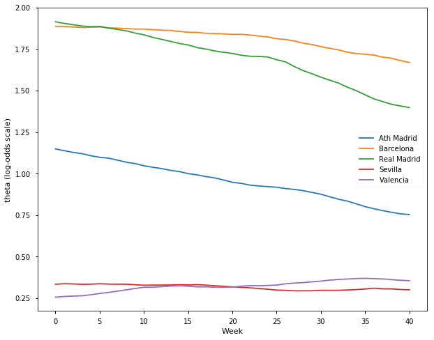
plot_final_rating(samplesS1718, TeamsS1718)
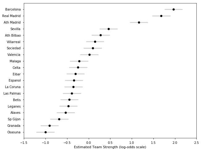
## Spanish La Liga Season 2016-17
samplesS1617, TeamsS1617 = get_results('SP1617.csv', l)
INFO:pystan:COMPILING THE C++ CODE FOR MODEL anon_model_7eab52f40be587905f219e2d7f11fcab NOW.
WARNING:pystan:9 of 4000 iterations saturated the maximum tree depth of 10 (0.225%)
WARNING:pystan:Run again with max_treedepth larger than 10 to avoid saturation
WARNING:pystan:Chain 1: E-BFMI = 0.11452305964640759
WARNING:pystan:Chain 2: E-BFMI = 0.11288825810124906
WARNING:pystan:E-BFMI below 0.2 indicates you may need to reparameterize your model
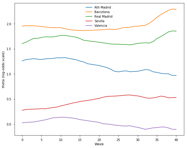
plot_final_rating(samplesS1617, TeamsS1617)
## Spanish La Liga Season 2015-16
samplesS1516, TeamsS1516 = get_results('SP201516.csv', l)
INFO:pystan:COMPILING THE C++ CODE FOR MODEL anon_model_7eab52f40be587905f219e2d7f11fcab NOW.
WARNING:pystan:14 of 4000 iterations saturated the maximum tree depth of 10 (0.35%)
WARNING:pystan:Run again with max_treedepth larger than 10 to avoid saturation
WARNING:pystan:Chain 1: E-BFMI = 0.04952938141672295
WARNING:pystan:Chain 2: E-BFMI = 0.0809009950131426
WARNING:pystan:E-BFMI below 0.2 indicates you may need to reparameterize your model
plot_final_rating(samplesS1516, TeamsS1516)
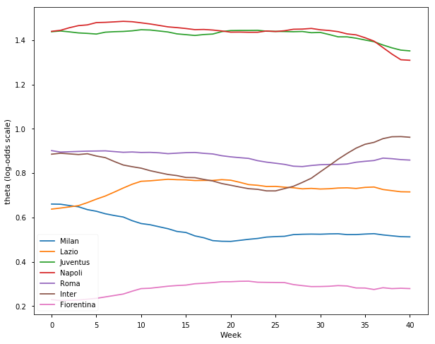
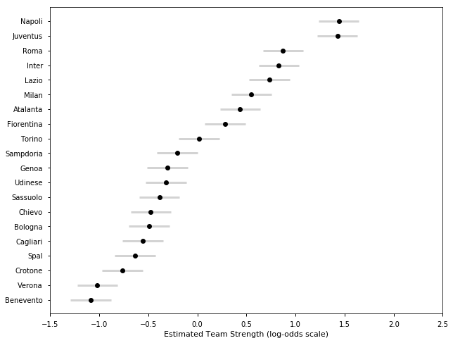
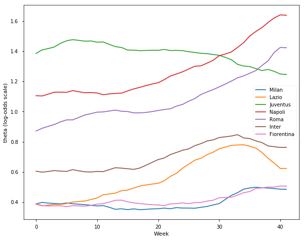
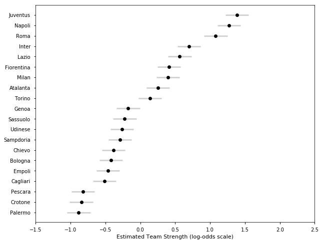
## Italian Serie-A Season 2017-18
l = ['Milan', 'Lazio', 'Juventus', 'Napoli', 'Roma', 'Inter', 'Fiorentina']
samplesI1718, TeamsI1718 = get_results('I201718.csv', l)
INFO:pystan:COMPILING THE C++ CODE FOR MODEL anon_model_7eab52f40be587905f219e2d7f11fcab NOW.
WARNING:pystan:Rhat for parameter tauWeek is 1.1417072632226644!
WARNING:pystan:Rhat for parameter lp__ is 1.1472510615694864!
WARNING:pystan:Rhat above 1.1 or below 0.9 indicates that the chains very likely have not mixed
WARNING:pystan:32 of 4000 iterations saturated the maximum tree depth of 10 (0.8%)
WARNING:pystan:Run again with max_treedepth larger than 10 to avoid saturation
WARNING:pystan:Chain 1: E-BFMI = 0.01542125656995636
WARNING:pystan:Chain 2: E-BFMI = 0.05116209221055198
WARNING:pystan:E-BFMI below 0.2 indicates you may need to reparameterize your model
plot_final_rating(samplesI1718, TeamsI1718)
## Italian Serie A Season 2016-17
samplesI1617, TeamsI1617 = get_results('I201617.csv', l)
INFO:pystan:COMPILING THE C++ CODE FOR MODEL anon_model_7eab52f40be587905f219e2d7f11fcab NOW.
WARNING:pystan:2 of 4000 iterations saturated the maximum tree depth of 10 (0.05%)
WARNING:pystan:Run again with max_treedepth larger than 10 to avoid saturation
WARNING:pystan:Chain 1: E-BFMI = 0.09936747025562734
WARNING:pystan:Chain 2: E-BFMI = 0.10194066305039481
WARNING:pystan:E-BFMI below 0.2 indicates you may need to reparameterize your model
plot_final_rating(samplesI1617, TeamsI1617)
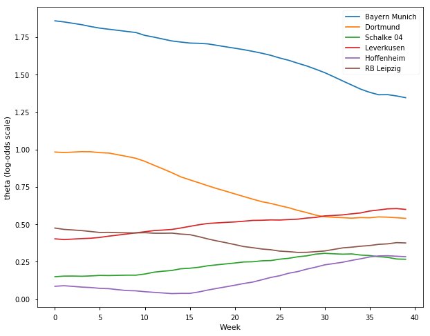
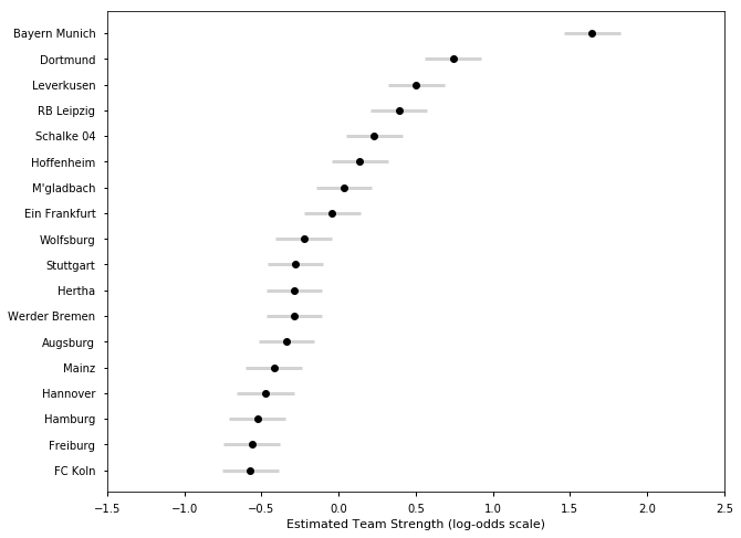
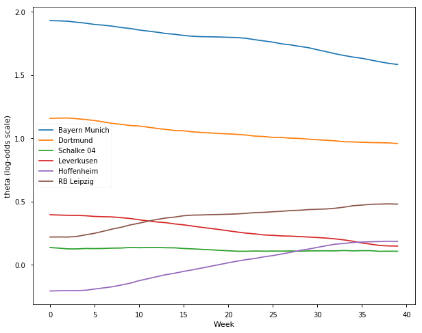
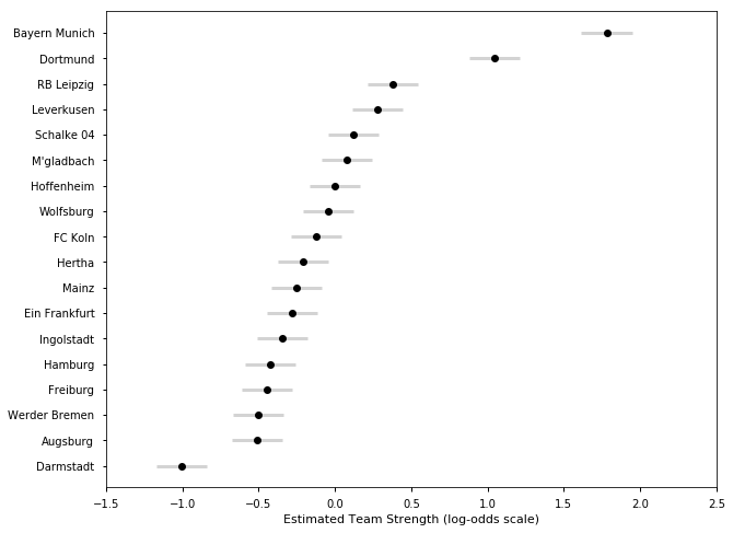
## German Bundesliga Season 2017-18
l = ['Bayern Munich', 'Dortmund', 'Schalke 04', 'Leverkusen', 'Hoffenheim', 'RB Leipzig']
samplesG1718, TeamsG1718 = get_results('G201718.csv', l)
INFO:pystan:COMPILING THE C++ CODE FOR MODEL anon_model_7eab52f40be587905f219e2d7f11fcab NOW.
WARNING:pystan:78 of 4000 iterations saturated the maximum tree depth of 10 (1.95%)
WARNING:pystan:Run again with max_treedepth larger than 10 to avoid saturation
WARNING:pystan:Chain 1: E-BFMI = 0.04827427484378621
WARNING:pystan:Chain 2: E-BFMI = 0.03491851795304218
WARNING:pystan:E-BFMI below 0.2 indicates you may need to reparameterize your model
plot_final_rating(samplesG1718, TeamsG1718)
## German Bundesliga Season 2016-17
samplesG1617, TeamsG1617 = get_results('G201617.csv', l)
INFO:pystan:COMPILING THE C++ CODE FOR MODEL anon_model_7eab52f40be587905f219e2d7f11fcab NOW.
WARNING:pystan:Rhat for parameter tauWeek is 1.1031507075838558!
WARNING:pystan:Rhat for parameter lp__ is 1.1105726053896596!
WARNING:pystan:Rhat above 1.1 or below 0.9 indicates that the chains very likely have not mixed
WARNING:pystan:60 of 4000 iterations saturated the maximum tree depth of 10 (1.5%)
WARNING:pystan:Run again with max_treedepth larger than 10 to avoid saturation
WARNING:pystan:Chain 1: E-BFMI = 0.04050288658515058
WARNING:pystan:Chain 2: E-BFMI = 0.03558983763290536
WARNING:pystan:E-BFMI below 0.2 indicates you may need to reparameterize your model
plot_final_rating(samplesG1617, TeamsG1617)
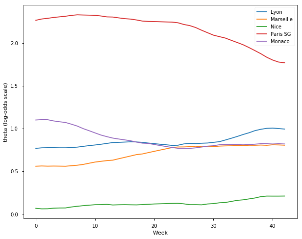
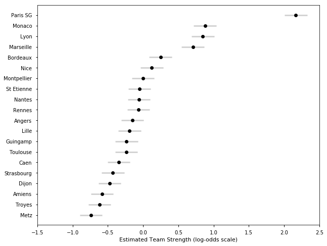
## French Ligue Un Season 2017-18
l = ['Lyon', 'Marseille', 'Nice', 'Paris SG', 'Monaco']
samplesF1718, TeamsF1718 = get_results('F201718.csv', l)
INFO:pystan:COMPILING THE C++ CODE FOR MODEL anon_model_7eab52f40be587905f219e2d7f11fcab NOW.
WARNING:pystan:22 of 4000 iterations saturated the maximum tree depth of 10 (0.55%)
WARNING:pystan:Run again with max_treedepth larger than 10 to avoid saturation
WARNING:pystan:Chain 1: E-BFMI = 0.05679069995578557
WARNING:pystan:Chain 2: E-BFMI = 0.038220014082986746
WARNING:pystan:E-BFMI below 0.2 indicates you may need to reparameterize your model
plot_final_rating(samplesF1718, TeamsF1718)
## French Ligue Un Season 2016-17
samplesF1617, TeamsF1617 = get_results('F201617.csv', l)
INFO:pystan:COMPILING THE C++ CODE FOR MODEL anon_model_7eab52f40be587905f219e2d7f11fcab NOW.
WARNING:pystan:27 of 4000 iterations saturated the maximum tree depth of 10 (0.675%)
WARNING:pystan:Run again with max_treedepth larger than 10 to avoid saturation
WARNING:pystan:Chain 1: E-BFMI = 0.06401256807721244
WARNING:pystan:Chain 2: E-BFMI = 0.057216887359233
WARNING:pystan:E-BFMI below 0.2 indicates you may need to reparameterize your model
plot_final_rating(samplesF1617, TeamsF1617)
Comparing Team Strength Across Leagues
def plot_comp_rating(s, Ts):

    plt.figure(figsize = (10,20))
    data = []
    for samples, Teams in zip(s, Ts):
        x = samples['theta'][1000:][35:][:].mean(axis = 0).mean(axis=0)
        e = samples['theta'][1000:][35:][:].std(axis = 0).mean(axis=0)

        data.extend(sorted(list(zip(x, Teams, e)), key = lambda x: x[0]))

    x_val = [x[0] for x in data]
    e_val = [x[2] for x in data]
    T = [x[1] for x in data]

    x = x_val
    y = np.linspace(-2, 2, len(data))
    my_yticks = T

    plt.yticks(y, my_yticks)
    plt.errorbar(x, y[:len(x_val)], xerr = e_val, fmt='o', color='black',
                 ecolor='lightgray', elinewidth=3, capsize=0)
    plt.xlabel('Estimated Team Strength 2016/17 (log-odds scale)')
    plt.xlim(-1.5,2.5)
    plt.savefig('TeamRating1617.png', dpi = 300, bbox_inches = 'tight')
    plt.show()
s = [samplesE1718, samplesS1718, samplesG1718, samplesI1718]
Ts = [TeamsE1718, TeamsS1718, TeamsG1718, TeamsI1718]

plot_comp_rating(s, Ts)
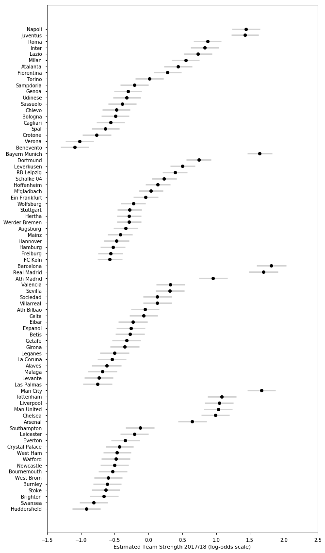
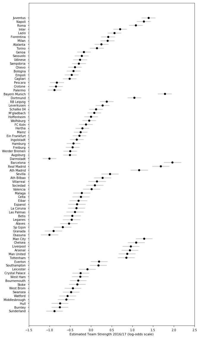
The plot above shows the team strength rating in the final week of the season. Plotting it in the way I have done above allows us to also compare competitiveness across leagues. It appears that the gap between the best and the worst teams is larger in Italy, Spain and Germany than in England. Teams 2-6 in England appear to be better than peers in all other leagues. The bottom 7 or 8 teams appear to be equally bad in all other leagues. The difference between the best and teams 2-6 in the Premier League is also more pronounced in 2017-18 than it used to be, considering Manchester City had a historic season recording 100 points. The plot below does the same for season 2016-17 and you can see that the difference is not as pronounced.
## Season 2016-17
s = [samplesE1617, samplesS1617, samplesG1617, samplesI1617]
Ts = [TeamsE1617, TeamsS1617, TeamsG1617, TeamsI1617]

plot_comp_rating(s, Ts)
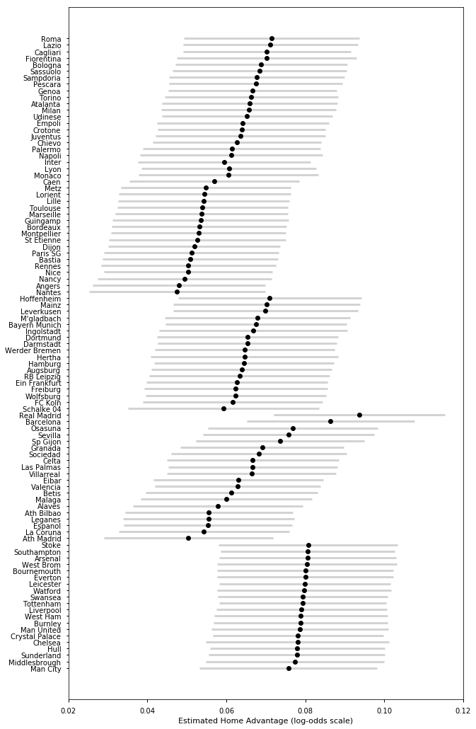
Comparing Home Advantage
def plot_home_adv(s, Ts):

    plt.figure(figsize = (10,18))
    data = []
    #plt.figure.tight_layout()
    for samples, Teams in zip(s, Ts):
        x = samples['alphaTeam'][1000:][:].mean(axis = 0) + samples['alpha'].mean(axis = 0)
        e = samples['alphaTeam'][1000:][:].std(axis = 0)

        data.extend(sorted(list(zip(x, Teams, e)), key = lambda x: x[0]))

    x_val = [x[0] for x in data]
    e_val = [x[2] for x in data]
    T = [x[1] for x in data]

    x = x_val
    y = np.linspace(-2, 2, len(data))
    my_yticks = T

    plt.yticks(y, my_yticks)
    plt.errorbar(x, y[:len(x_val)], xerr = e_val, fmt='o', color='black',
                 ecolor='lightgray', elinewidth=3, capsize=0)
    plt.xlabel('Estimated Home Advantage (log-odds scale)')
    plt.xlim(0.02,0.12)
    plt.savefig('1617HomeStrength.png', dpi = 300, bbox_inches = 'tight')
    plt.show()
s = [samplesE1617, samplesS1617, samplesG1617, samplesF1617, samplesI1617]
Ts = [TeamsE1617, TeamsS1617, TeamsG1617, TeamsF1617, TeamsI1617]

plot_home_adv(s, Ts)
s = [samplesE1718, samplesS1718, samplesG1718, samplesF1718, samplesI1718]
Ts = [TeamsE1718, TeamsS1718, TeamsG1718, TeamsF1718, TeamsI1718]

plot_home_adv(s, Ts)
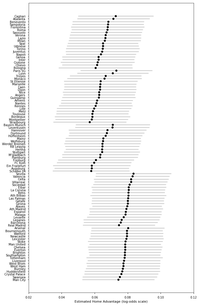
Looking at the above two plots, it appears there is a small home advantage. It is the highest in the English Premier League on average compared to the other leagues. This might explain why the Premier League is more competitive than the other leagues.